Quick Review: Big-O Notation
As a web developer, I very rarely find myself deeply analyzing algorithms. However, a basic understanding of Big-O analysis can be really useful for software engineers. It provides a common language for us to discuss the performance of our code and the potential ways we can improve it.
What is Big-O notation?
An algorithm is a set of operations describing how to solve a problem. Generally, the more complex an algorithm, the longer it takes to run. How do we describe an algorithm’s complexity?
Big-O notation is a way to express an algorithm’s complexity in terms of the size of its input. It gives us an idea of how an algorithm scales as its input grows. An algorithm can be classified into one of several Big-O functions, usually written as O(n) or O(n2). With these functions, we can compare the complexity (and performance) of our algorithms.
A Basic Example
Here’s a simple search function:
def linear_search(target, items):
  for item in items:
    if target == item:
      return True
  return False
Let’s walk through the steps for determining this function’s Big-O complexity:
Determine the Input Size
This one is relatively simple: the number of elements in items is our input size, n.
Only Consider the Worst-Case Scenario
If the first item in items is equal to target, the function returns in only one operation. This is the best-case scenario. We only care about the worst-case scenario, which occurs when target doesn’t exist in items at all. In this situation, we end up iterating through the entire list.
Count the Number of Operations
We can express the number of operations performed as a function of n. We know our worst-case scenario involves iterating the entire list. So, the Big-O complexity of linear_search is O(n). In other words, our algorithm completes in “linear time”. If items has 10 items, we do 10 operations. If it has 1000 items, we do 1000 operations. And so on.
Ignore Insignificant Terms
Big-O notation is an approximation on large values of n. This means as n gets extremely large, some terms end up being less significant than others. So, we just drop them. Also, we are evaluating operations without any specific unit of “cost”. This means coefficients aren’t very meaningful. We can drop them as well.
For example:
O(23n2 + 45n + 100000)
is reduced to
O(n2)
Common Big-O Classes
With a basic understanding of Big-O analysis, let’s look at some common classes of complexities:
O(1)
This is known as “constant time” because the algorithm completes in the same amount of time no matter what the size of the input is. An example of this is pushing or popping from a stack:
def push(item, items):
  items[len(items):] = [x]

def pop(items)
  item = items[-1]
  del items[-1]
  return item
Regardless of how big items is, we still yield the same amount of operations.
O(log(n))
Let’s revisit our searching algorithm from before. What if we assumed our input is sorted? With this assumption, we can reduce the runtime complexity of our search by taking a different approach:
def binary_search(target, sorted_items):
  if len(sorted_items) == 0:
    return False
  else:
    mid = len(sorted_items) / 2

    if sorted_items[mid] == target:
      return True

    if target < sorted_items[mid]:
      return binary_search(target, sorted_items[:mid])
    else:
      return binary_search(target, sorted_items[mid+1:])
This approach is commonly known as “divide and conquer”. Rather than looping through all items, divide-and-conquer algorithms halve the input size (often recursively) at each step.
This results in an algorithmic complexity resembling a logarithmic function, thus the Big-O complexity of O(log(n)).
O(nlog(n))
Some algorithms involve some kind of divide-and-conquer strategy combined with linear processing of all elements. This is very common in sorting algorithms. An example of this is merge_sort:
def merge_sort(items):
  if len(items) > 1:
    mid = len(items) / 2
    left = merge_sort(items[:mid])
    right = merge_sort(items[mid:])

    return merge(left, right)
  else:
    return items

def merge(left, right):
  new_array = []

  while len(left) > 0 and len(right) > 0:
    if left[0] < right[0]:
      new_array.append(left.pop(0))
    else:
      new_array.append(right.pop(0))

  while len(left) > 0:
    new_array.append(left.pop(0))
  while len(right) > 0:
    new_array.append(right.pop(0))

  return new_array
In merge_sort, we implement our divide-and-conquer strategy. As we’ve learned, this has a runtime complexity of O(log(n)).
The “merging” occurs in merge. In this function, we compare the heads of each array, popping the smaller element, and pushing it into a new array. The result is a merged, sorted array. Since we process each element in both arrays, this function has a runtime complexity of O(n).
When all is said in done, we get an overall runtime complexity of O(nlog(n)).
O(nx)
A big clue to identifying algorithms with O(nx) complexity is nested loops. We usually say these algorithms complete in “polynomial time”. Inefficient sorting algorithms often fall into this class:
def bubble_sort(items):
  for i in range(0, len(items)):
    for j in range(0, len(items)):
      if items[i] <= items[j]:
        tmp = items[i]
        items[i] = items[j]
        items[j] = tmp
  return items
In bubble_sort, for each item in items, we make another iteration back over items and swap elements according to their value. This “bubbles up” each item to its correct position in the array. Since there is a loop within a loop, this function yields total of n * n operations. This means the Big-O complexity of bubble_sort is O(n * n), or O(n2).
Visualizing Big-O
We can easily compare different Big-O complexities by graphing them:
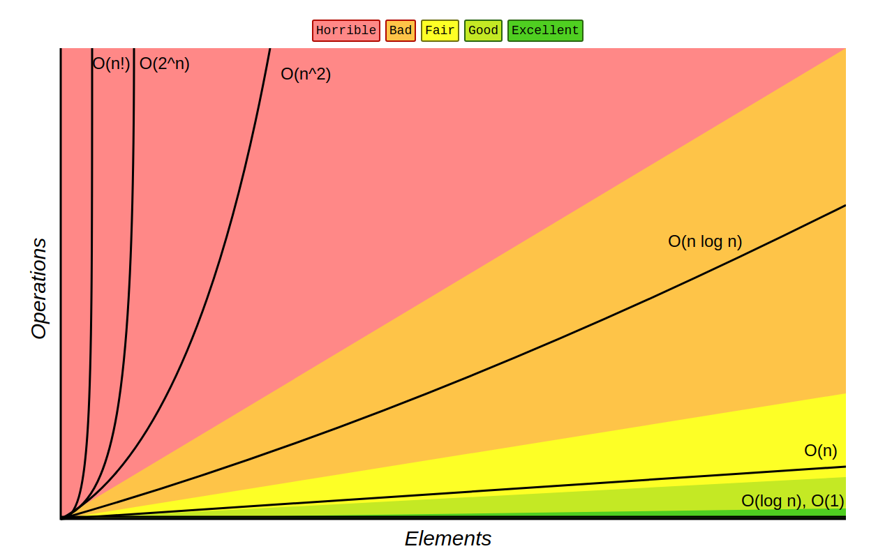
(Source: http://bigocheatsheet.com/)
If it can be helped, we should strive to write functions with complexities O(nlog(n)) or better. These classes of algorithms scale much better than their polynomial and exponential counterparts.
Conclusion
Obviously, this is a very basic explanation for Big-O notation. There’s much more math involved in describing and proving these concepts. Here are some great resources for learning more about Big-O notation and analysis:
- Big O Notation by Interview Cake
- Big-O notation explained by a self-taught programmer by Justin Abrahms
- Learning and Understanding Big-O Notation by Topcoder
- Big O notation by Wikipedia
Questions? Comments? Corrections? Please let me know below!